Methods
The purpose of this research was to understand patterns of health service use by ex-serving members in the last year before death by suicide. To achieve this, the research was undertaken in three stages
- Comparative analysis which contrasted health service use between those who died by suicide and matched controls, establishing the odds of health service use associated with suicide death across different service types.
- Cluster analysis (latent class analysis) of those who died by suicide to identify subgroups of persons based on patterns of service use in the last year of life.
- Trend analysis (group-based trajectory analysis) which examined how health service use patterns evolved over time during the year before death by suicide, identifying trajectories of service use intensity and critical periods for intervention.
This multi-stage analytical approach provided complementary insights capturing differences in service use between those who died by suicide and matched controls, patterns of engagement among cases and changes in service use over time for cases in the last year of life.
Health service use in the last year of life compared with those who did not die by suicide
For the first stage AIHW used a statistical approach that would enable comparisons of health service use between those who died by suicide and those who did not, while accounting for confounding factors known to influence service use such as age, sex, socioeconomic status and geographic location. By adjusting for these factors, the outputs more accurately represent differences in service use that may be associated with death by suicide, rather than differences due to sociodemographic or health-related characteristics.
The study population consisted of ex-serving ADF members aged 17 years and older who died by suicide between 1 July 2011 and 30 June 2020 excluding deaths in Western Australia and Northern Territory (due to limited public hospital data). Death by suicide was defined as the principal external cause of death in X60-X84 and Y87.0 based on the ICD-10 codes (AIHW 2022).
For each case, the index date was set as the date of death. There was a secondary study population used for the analysis where diagnostic information in ED care was required. This was ex-serving ADF members aged 17 years and older who died by suicide between 1 July 2014 and 30 June 2020. This population was used because of limited diagnostic information in ED care prior to this time.
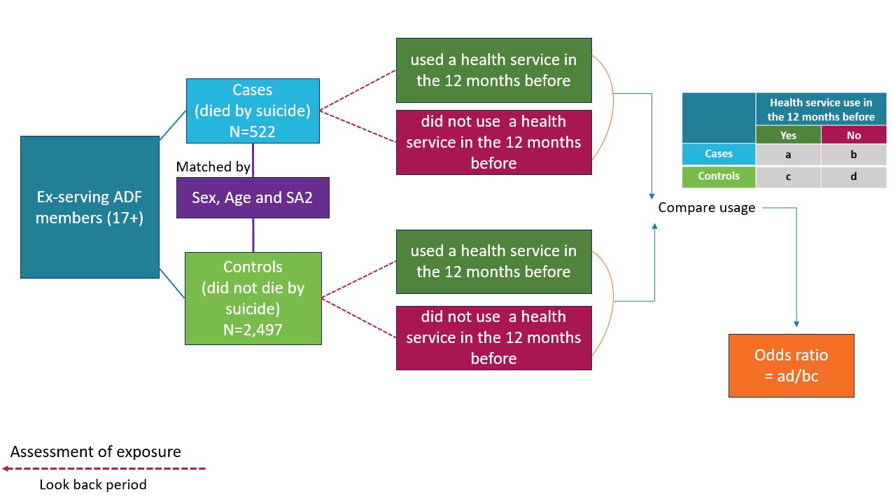
The approach used by AIHW was to assess how patterns of health service use may differ between those who died by suicide (cases) and matched controls who did not die by suicide. This helps identify service settings or time points where earlier intervention may be possible. In this study, cases (ex-serving members who died by suicide) were matched with controls (ex-serving members who were alive). Figure 12 shows the study design. The matching process involved ensuring that persons in the control group were the same sex, a similar age and resided in a similar location (to account for variations in socioeconomic status and access to health services).
The comparison population were ex-serving ADF members aged 17 years and older who were either alive or died of other causes, but all were alive at the time of the cases’ death and survived for at least one year afterward. Using live controls enables comparability in exposure periods, minimising bias related to survival time. This approach helps in identifying differences in health service use and other characteristics between those who died by suicide and those who did not.
Up to five controls were randomly matched to cases based on sex, age (using ±5 birth years) and Statistical Area Level 2 (SA2) at the index date (case’s date of death) to ensure comparability and reduce confounding effects. Controls were uniquely matched to cases without replacement. For the small proportion of cases (0.9%), that could not be matched by SA2, a secondary matching by ensuring the same socioeconomic status (Index of Relative Socio-economic Disadvantage (IRSD) decile) and remoteness category within the same state was performed to maintain comparability (ABS 2018a; ABS 2018b). A 1:5 case-control matching ratio was initially targeted, with 96.4% of cases matched to at least 3 controls, 3.6% matched to two controls or 1 control. This varied ratio was retained to ensure that cases with limited available matches were included, preserving 99% of the case cohort, thereby ensuring a representative sample, while maintaining comparability and statistical power.
Figure 12: Study design
Types of health services used
The analysis included five types of health services based on the different data sources for each service type. These were:
- primary care services (MBS) including general practitioner services, specialists, allied health, operations, and diagnostic services such as pathology and diagnostic imaging
- Pharmaceuticals (PBS/RPBS)
- Admitted hospital care including DVA-funded services
- Emergency department care including DVA-funded services
- DVA-funded primary care services (MBS equivalent services).
Each of these service types was split into mental health and non-mental health categories (see Classifications and codes). Further disaggregation such as injury admitted care, GP and specialists were undertaken where possible. The definition for each of the analysed service types and subcategories are outlined in Table 3.
For each service type, health service use in the last year was examined over multiple timepoints prior to the index date (the date of death by suicide and equivalent date for matched controls). The timepoints included the final week, final month, three months, six months, nine months, and the year before to capture both short-term and longer-term patterns of service use, and to identify periods that may be appropriate for intervention. Any hospital episode (ED presentation, hospital admission) that ended in “death” was excluded as it was considered to be a result of the fatal (suicide) incident (Clapperton et al. 2021). Any health services accessed on the index date were excluded from the analysis (Ahmedani et al 2019; DelPozo-Banos et al. 2024; John et al. 2020).
Statistical methods
The first part of this analysis was descriptive analysis to outline the characteristics of cases and controls as well as to identify the proportion of each group that accessed each health service type and the frequency that each health service was used in the last year of life for those who died by suicide or equivalent year for those who remained alive.
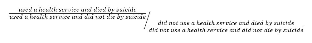
The second component of the analysis used a conditional logistic regression model to estimate odds ratio (OR). These describe the likelihood of ex-serving members who died by suicide having accessed a health service compared to other matched ex-serving members who did not die by suicide. OR were calculated for each health service type, with 95% confidence intervals (CI), based on matched case-control pairs.
The ORs do not reflect the risk or probability of dying by suicide, nor do they indicate whether health services caused or prevented suicide. Instead, they describe how common health service use was among cases relative to controls. An OR greater than 1 indicates that cases were more likely to have accessed a particular health service than matched controls; an OR less than 1 indicates cases were less likely to have accessed that health service.
The formula for the OR is outlined below.
Controlling for confounding effects
As mentioned above, matching performed in the case-control study was used to account for differences in sociodemographic factors between those died by suicide and those who remained alive. This included sex, age and location (as a proxy for socioeconomic status and health services accessibility). This approach will minimise differences in these characteristics between the groups. However, other important differences between the two groups are likely to remain. This will include differences in the underlying health of the two groups (comorbidities, see described below), which is likely to be strongly related to the outcomes assessed in this report and was thus controlled for in the modelling.
Area-level measures
AIHW used SA2 as the location variable sourced from the Medicare Consumer Directory to account for differences in socioeconomic characteristics and remoteness (which is likely to be strongly related to access to health services) between the groups. This included using Australian Bureau of Statistics (ABS) sourced Socio-Economic Indexes For Areas (ABS 2018a), remoteness classifications (using ABS Remoteness Areas, ABS 2018b) and the calculation of a health service accessibility index based on shortest travel times to health services from SA2s. This approach enabled AIHW to describe variation in health service use in relation to geographic and socioeconomic factors. However, AIHW notes that applying these characteristics from a SA2 are a proxy and that individual record data would be more precise to understand these impacts on health service use.
In this report, the five categories of ABS remoteness were collapsed into two: major cities and regional/remote areas (inner regional, outer regional, remote and very remote areas).
Socioeconomic status was defined by the IRSD quintiles, which were collapsed into three categories: low (first quintile), mid (second-fourth quintile), and high (fifth quintile).
Health service accessibility was measured using the health service accessibility index. This index is a percentile ranking that measures accessibility to key health services across SA2 regions. It is based on the shortest travel time to hospitals, emergency departments, mental health services, pharmacies and general practitioners. The index ranges from 0 to 1, where lower values indicate better accessibility (shorter travel times) and higher values indicate poorer accessibility (longer travel times). The index was divided into quartiles for analysis, categorising areas as most accessible, moderately accessible, less accessible, and least accessible.
Multimorbidity
There were two co-morbidity indices used to adjust for the presence or absence of comorbidities at one year prior to the index date.
The RxRisk comorbidity index is based on prescription medicines use (PBS/RPBS), and captures 46 selected chronic conditions using Anatomic Therapeutic Chemical (ATC) codes for prescribed medications (Pratt et al 2018). A one-year lookback period prior to the index date was used to capture active comorbid conditions. A single prescription for any specified medication within each condition category was considered indicative of the presence of that condition. In this report, the weighted scores for 46 comorbid conditions as described by Pratt et al 2018 was used. The RxRisk Index was categorised as 0 (no comorbidities), 1 (moderate comorbidity burden) and 2+ (high comorbidity burden)
The Multipurpose Australian Comorbidity Scoring System (MACSS) based on principal and additional hospital diagnosis codes (admitted patient care), captures 102 selected comorbid conditions using the ICD10-AM codes (Homan et al 2005; Toson et al 2016). Each comorbid condition was flagged as absent or present based on a one-year look back period prior to the index date. The number of MACSS comorbidities was categorized as none, one, or two or more conditions.
Using both indices allowed for a more comprehensive adjustment for comorbidities, capturing both medication usage and hospital-diagnosed conditions. Caution is advised when interpreting the adjusted results for PBS services, hospital services and any health service use, as the comorbidity indices (RxRisk Index from PBS/RPBS data and MACSS index from hospital data) were derived from these same data sources. As comorbidity indices used for adjustment in the conditional logistic regression model included mental health conditions and were measured over the same 12-month period as the health service use outcomes, some over-adjustment of the modelled odds ratios may have occurred.
Continuity and regularity of GP care
Continuity of GP care was measured using the Usual Provider of Care (UPC) index, which calculates the proportion of GP visits (identified based on MBS item numbers, date of service and provider number) a patient has with their most usual GP (Welsh et al 2023). UPC as a measure of relational continuity of care was calculated using the formula:
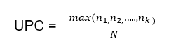
Where max (n1, n2,…nk) is the number of visits to the GP with whom the patient had the greatest number of visits, and N is the total number of visits by the patient to all providers during the same period. The UPC index reflects relational continuity with the same GP but does not capture continuity within a practice, which may also benefit patient care.
Regularity of GP care was measured using the Modified Regularity Index (MRI), which assesses the distribution of GP visits over time, based on the variation in the number of days between GP visits, with more even dispersion indicating better regularity (or planned, proactive care (Welsh et al 2023). MRI was calculated using the formula:
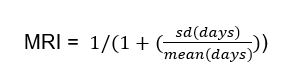
Both UPC and MRI were calculated for cases and controls with at least three GP visits in the 12 months before the index date, ensuring sufficient data to accurately access continuity and regularity of care (Dreiher et al 2012). Both UPC and MRI result in scores ranging from 0 to 1. The UPC index was categorised into five groups: low (index range 0–0.49), moderate (0.5–0.74), high (0.75–0.99) and perfect (1) continuity and those without a UPC index categorised separately. For analysis, the UPC categories were then dichotomised into poor continuity (low and moderate) and high continuity (high and perfect). The MRI was categorised into quintiles (least to most regular), with an additional category for those without an MRI score. For analysis, the MRI quintiles were then dichotomised into poor regularity (quintiles 1-3) and high regularity (quintiles 4 and 5).
Identifying groups of ex-serving members who died by suicide by their health services use in the last year of life
For the second stage of the analysis AIHW used a statistical approach referred to as latent class analysis (LCA) to identify subgroups based on health service use patterns over a person’s last year of life.
LCA was selected over other clustering methods (such as k-means, hierarchical clustering) due to its statistical robustness and model-based approach to identify health service use patterns. LCA provides objective fit statistics, estimates membership probabilities for class selection rather than forced classification, and better handles mixed data types, resulting in more reliable pattern identification. Studies have shown that LCA produces lower misclassification rates compared to traditional clustering methods, making it particularly suitable for identifying complex health service use patterns (Naldi et al 2020).
The study population consisted of ex-serving ADF members aged 17 years and older who died by suicide between 1 July 2014 and 30 June 2020. Only the data back to 2014 was used as a result of limitations with ED data between 2010 and 2013. However, the ex-serving population who died between 1 July 2011 and 30 June 2020 and the LCA cohort had similar demographic and service-related profiles, suggesting that the limitation to the cohort did not affect the representativeness of the patterns identified. The population that was analysed using this method was limited to ex-serving members who died by suicide to better understand health service use patterns preceding death by suicide, helping guide future intervention strategies. However, Health service use among ex-serving ADF members provides information on LCA performed on the total ex-serving population.
Statistical methods
The first part of the analysis was developing the LCA model to allocate deceased ex-serving members to a group. This process is explained in the next section. Following this, the analysis focussed on describing the characteristics of persons in each group and the number and type of health services used by the study population in the year before death. The health services that were included in the analysis were: mental health contact (MBS and ED/hospital), non-mental health contact (MBS and ED/hospital), investigation (such as diagnostic procedures, diagnostic imaging, and pathology from MBS), mental health medicine dispensed (PBS/RPBS), and non-mental health medicine dispensed (PBS/RPBS).
Latent class analysis
LCA was used to identify distinct subgroups based on health service use among ex-serving members who died by suicide from 1 July 2013 to 30 June 2019 (1-year before death). LCA is a data-driven model-based approach that identifies underlying subgroups (called latent classes or groups) based on multiple observed variables (indicators). Individuals are probabilistically assigned to the groups based on two model parameters estimated on a maximum-likelihood basis:
- group membership probabilities
- the means and variances of the indicator variables, conditional on group membership.
Groups of individuals sharing similar patterns of the means and variances of each indicator variable are identified and grouped. This enables the distinctness of each identified groups to be assessed and qualitatively described.
The model building process to determine the optimal number of latent groups was iterative. Models with increasing number of groups (up to seven) were fitted. The best-fitting model with the optimal number of groups was selected using several criteria:
- relative fit statistics (Akaike Information Criterion and Bayesian Information Criterion)
- classification diagnostics (entropy values close to 1, average posterior probability of group membership > 0.7 for each group, odds of correct classification based on posterior probabilities > 5 for each group and close correspondence between each group’s estimated probability of group membership and the proportion of cases classified to that group according to posterior probability of group membership)
- smallest group size greater than 5% of the sample
- substantive model interpretability and parsimony.
Models were estimated with 30 Expectation-Maximisation iterations and 50 draws of random starting values to ensure that a global rather than a local (sub-optimal) solution was found.
The stability of the chosen number of groups across different random samples of the data was tested using a five-fold cross validation approach by randomly splitting the data into five subsets and conducting a LCA analysis on each subset. The consistency of the results in terms of group size information across the five subsets confirmed the robustness of the optimal number of group and validated the reliability of the modelling approach.
Once latent groups were identified, multinomial logistic regression was used to examine how individual and service level variables (independent variables) predicted group membership (dependent variable). The coefficients from the regression models were exponentiated to obtain relative risk ratios (RRR) with 95% confidence intervals (CI).
The characteristics of ex-serving members who died by suicide and the identified latent groups were summarised using frequencies and percentages. Chi-squared tests were used to assess the differences in distributions of individual and service characteristics across the identified groups.
Health service use trends during the last year of life
The third stage of the analysis included examination of the trends in health service use during the last year of life for ex-serving members who died by suicide. It focussed on identifying different patterns or trajectories of use during the year to find opportunities for intervention using group-based trajectory modelling (GBTM).
Like LCA, GBTM provides a model-based, probabilistic approach to identify distinct trajectories, but for longitudinal data. GBTM was chosen over other trajectory modelling techniques (such as Growth mixture modelling) for its simplicity and ease of interpretation. GBTM is known for providing clearer classification and more interpretable results (Den Teuling et al 2021; Lu 2024; Nguena et al 2020).
The study population consisted of ex-serving ADF members aged 17 years and older who died by suicide between 1 July 2014 and 30 June 2020 similar to the LCA due to limitations in earlier ED data and to focus on the cohort that could benefit from intervention.
Statistical methods
The number of health service contacts by type (mental health contact, physical health contact, investigation, mental health medicine dispensed, physical health medicine dispensed) per 30-day period for the twelve months prior to death by suicide was calculated (Chitty et al 2023). Following this, the GBTM was developed to allocate ex-serving members to a group. This process is explained in the next section.
The analysis from GBTM outlines the number and type of health services used by the study population in the year before death as well as describing the characteristics of each group across each health service type.
Group-based trajectory modelling
Group-based trajectory modelling (GBTM) was used to identify trajectories of health service use among ex-serving members who died by suicide between 1 July 2014 and 30 June 2020 and their health service use in the last year of life. GBTM provides a statistical method to identify groups of separate trajectories that are summarised by a finite set of different polynomial functions of time as per maximum likelihood estimation.
The number of services that the decedent used per month in the last year of life was modelled as a zero-inflated Poisson distribution (Schneider et al 2020). With this approach, trajectories were estimated by the model, and every decedent was assigned a probability of belonging to each trajectory, with total probability of membership summing up to 1. We then used maximum probability assignment to determine group membership. The shapes of each trajectory were defined by polynomial terms (linear, quadratic or cubic).
The model building process to determine the optimal number of trajectories was iterative. First, the optimal number of groups were determined by iteratively testing models with one to five groups. The maximum number of groups was limited to five for avoiding small size trajectory groups and for interpretability of trajectories. The best-fitting model with the optimal number of trajectories was based on multiple criteria (Lennon et al 2018):
- relative fit statistics (Akaike Information Criterion and Bayesian Information Criterion)
- classification diagnostics (entropy values close to 1, average posterior probability of class membership > 0.7, odds of correct classification based on posterior probabilities > 5 for each trajectory group)
- smallest class size greater than 5% of the sample
- substantive model interpretability and parsimony.
Once the number of groups was determined, the next step involved selecting the optimal polynomial order for each group. For this, models were initially run with a quadratic order for all groups. The polynomial order (linear, quadratic or cubic) was then adjusted iteratively for each group to assess which combination provided the best fit according to the criteria mentioned earlier, with a preference for models that maximised BIC (closer to 0). Finally, individuals were assigned to a trajectory group based on their maximum posterior probabilities.
Model robustness was assessed using a five-fold cross validation (where the data was randomly split into five subsets and GBTM conducted on each subset), and bootstrap resampling with 1,000 replications. The stability and reliability of group membership was confirmed by comparing the group membership proportions across cross-validation folds against observed and expected proportions and their 95% confidence intervals from bootstrapping.
Once optimal trajectory models were selected, bivariate multinomial logistic regressions were conducted to identify characteristics associated with trajectory group membership, and relative risk ratios (RRR) with 95% confidence intervals (CIs) were reported.
The characteristics of the decedents and the identified trajectories were summarised using frequencies and percentages. Chi-squared test was used to assess the differences in distributions of individual and service characteristics across the identified trajectories.