Methods
The purpose of this research was to describe patterns of health service use by ex-serving members before and after a self-harm event, and compare health service among this group to a comparison group of ex-serving members. This study used a matched cohort study design to examine the change in health service use among ex-serving members in the 12 months before and after an index self-harm hospital admission (the first self-harm hospitalisation in the study period). The matched cohort study design is useful for assessing how use of health services are associated with self-harm risk, helping identify potential intervention points to prevent self-harm.
Study design
The study population (self-harm cohort) consisted of ex-serving ADF members aged 17 years and older who were admitted to public hospital for self-harm between 1 July 2011 and 30 June 2019 excluding admissions in Western Australia and Northern Territory. For each person in the self-harm cohort, the index date was set as the date of admission.
The first self-harm hospitalisation (the index hospitalisation) was identified based on the International Classification of Diseases, Australian Modification (ICD10-AM). Self-harm hospitalisations were identified using a principal diagnosis of injury (ICD10-AM: S00-T75 or T79) and the first reported external cause of self-harm (ICD10-AM: X60-X84, Y87.0) between 1 July 2011 and 30 June 2019. Index admissions occurred throughout this period.
In this study design, each ex-serving member in the self-harm cohort was matched with ex-serving members who were admitted to hospital for reasons other than injury, excluding both self-harm and non-self-harm injuries (the comparison cohort). Figure 10 shows the study design.
Figure 10: Matched cohort study design

Comparison cohort
Up to 5 persons from the admitted care dataset were randomly matched to each ex-serving member in the self-harm cohort based on sex, age (using ±5 birth years) and SA2 (to account for variations in socioeconomic status and access to health services) at the date of the index self-harm admission. Each matched comparison individual was then assigned the same index date as their matched self-harm counterpart to ensure temporal alignment for pre and post index analyses.
Each comparison individual was uniquely matched to an individual in the self-harm cohort without replacement. A 1:5 matching ratio was initially targeted, with 84.5% of those in the self-harm cohort matched to at least 3 comparators and 15.5% matched to 2 or 1 comparator. This varied ratio was retained to ensure that each person in the self-harm cohort was included, despite limited available matches, preserving 96.3% of the cohort and supporting statistical power.
The definition of the comparison cohort has impacts on the results presented in this report. The comparison cohort had demographic and service characteristics similar to the whole ex-serving population (AIHW 2024) and was matched to the self-harm cohort on key sociodemographic factors, and adjusted for comorbidities. However, important unmeasured differences likely remain between the two cohorts such as psychosocial or behavioural factors.
The comparison cohort did not include injury-related admissions to reduce misclassification of self-harm but this could also introduce bias by omitting individuals with overlapping risk profiles with those in the self-harm cohort. The comparison cohort includes a range of non-injury hospitalisations such as those related to chronic illness, mental health, and other conditions, contributing to heterogeneity in health profiles and healthcare needs. These factors should be considered when interpreting the patterns of health service use between cohorts.
Types of health services used
The analysis included five types of health services based on the different data sources for each service type. These were:
- Primary care services (MBS)
- Pharmaceuticals (PBS/RPBS)
- Admitted hospital care including DVA-funded services
- Emergency department care including DVA-funded services
- DVA-funded primary care services (MBS equivalent services).
Each of these service types was split into mental health and physical health. Further breakdowns such as GP and specialists were undertaken where possible. The definition for each of the analysed service types and subcategories are outlined in Table 4. All health services for the self-harm and comparison cohort were identified from 1 July 2010 to 30 June 2020. Any health services accessed on the index date were excluded from the analysis (Ahmedani et al 2019; DelPozo-Banos et al. 2024; Jakobsen et al 2025; John et al. 2020).
Statistical methods
The first part of this research was descriptive analysis to outline the characteristics of the self-harm and comparison cohort as well as to identify the proportion of each group that accessed each health service type and the frequency that each service was used in the year before and after the index admission.
Mortality within 12 months of index admission
The report also analysed the mortality of each cohort within 12 months of the index date. Mortality rates were estimated by following individuals from the index date until death or 12 months post index, whichever occurred first. Mortality rates were calculated as deaths per 1,000 person-years at risk. Using person years accounts for the survival time after the index admission to the date of death for the self-harm and comparison cohort (Mitchell and Cameron 2018).
To quantify mortality attributable to self-harm, the attributable risk percent (AR%) for mortality among the self-harm cohort was calculated using the below formula.
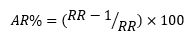
RR is the mortality rate ratio comparing the mortality rate in the self-harm cohort to the rate in the comparison cohort. The AR% represents the proportion of 12-month mortality within the self-harm cohort that may be attributable to self-harm, on the strong assumption that the only difference between two cohorts was the self-harm attempt.
Modelling health service use in the year before and after index admission
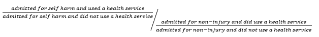
The aim of the second component of the analysis was to estimate odds ratio (OR) to describe differences in health service use between the self-harm and comparison cohort. OR were produced using generalised estimating equation (GEE) models along with 95% confidence intervals (CI) for the use of each healthcare service, among the matched cohort pairs.
The OR compare the odds of the outcome (health service use) in the self-harm cohort compared to the comparison cohort. If an OR is greater than 1 then it means that ex-serving members who were admitted for self-harm had higher odds of accessing a health service compared to those in the comparison cohort. Alternatively, if OR is below 1 then ex-serving members admitted for self-harm had lower odds of accessing the health service than those admitted for reasons other than injury. An OR of 1 indicates no differences in health service use between the two cohorts.
The formula for the OR is outlined below.
Higher OR do not imply a causal association between health service use and being admitted for self-harm; rather a higher odds indicates that those who were admitted for self-harm were more likely to access these services compared to the comparison cohort.
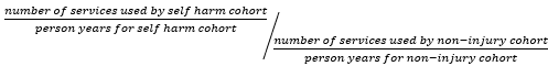
The analysis also included rate ratios (RR) to describe the frequency of using a health service between the self-harm and the comparison cohort. RR were produced using generalised estimating equation (GEE) models along with 95% confidence intervals (CI) for the rate (frequency) of each healthcare service, among the two cohorts. For these analyses, person years at risk were estimated as the time between the index hospital admission and death, or 12 months after the index admission (which ever occurred first).
The RR compares the rates of health service use in the self-harm cohort compared to the comparison cohort. If an RR is greater than 1 then it means that ex-serving members who were admitted for self-harm had higher rate of health service use compared to those in the comparison cohort. Alternatively, if RR is below 1 then ex-serving members admitted for self-harm had lower rates of health service use than those admitted for reasons other than injury. An RR of 1 indicates no differences in rates of health service use between the two cohorts.
The formula for the RR is outlined below.
A higher RR does not imply that frequent health service use causes self-harm. Rather, it indicates that individuals in the self-harm cohort used health services at a higher rate than those in the comparison cohort during the observed period.
Controlling for confounding effects
As mentioned above, matching was used to account for differences in basic demographics between those who were admitted for self-harm and the comparison cohort. This included sex, age and area of residence (as a proxy for socioeconomic status and health services accessibility). This approach minimises differences in these characteristics between the two cohorts. However, other important differences between the cohorts are likely to remain. This will include differences in the underlying health status of the two cohorts (comorbidities, see described below), which is likely to be strongly related to the outcomes (health service use and mortality) assessed in this report.
Area-level measures
AIHW used SA2 as the location variable sourced from the Medicare Consumer Directory to account for differences in socioeconomic characteristics and remoteness (which are likely to be strongly related to access to health services) between the two cohorts. This included using Australian Bureau of Statistics (ABS) sourced Socio-Economic Indexes For Areas (ABS 2018a), remoteness classifications (using ABS Remoteness Areas, ABS 2018b) and the calculation of a health service accessibility index based on shortest travel times to health services from SA2s. This approach enabled AIHW to describe variation in health service use in relation to geographic and socioeconomic factors. However, AIHW notes that applying these characteristics based on SA2 area of residence is an area-level measure that serves as a proxy and may not reflect individual-level socioeconomic status, which would provide more precise understanding of impacts on health service use.
In this report, the five categories of ABS remoteness were collapsed into two: major cities and regional/remote areas (inner regional, outer regional, remote and very remote areas).
Socioeconomic status was defined by the Index of Relative Socioeconomic Disadvantage area-based quintiles, which were collapsed into three categories: low (first quintile), mid (second-fourth quintile), and high (fifth quintile).
Health service accessibility was measured using the health service accessibility index. This index is a percentile ranking that measures accessibility to key health services across SA2 regions. It is based on the shortest travel time to hospitals, emergency departments, mental health services, pharmacies and general practitioners. The index ranges from 0 to 1, where lower values indicate better accessibility (shorter travel times) and higher values indicate poorer accessibility (longer travel times). The index was divided into quartiles for analysis, categorising areas as most accessible, moderately accessible, less accessible, and least accessible.
Multimorbidity
There were two co-morbidity indices used to adjust for the presence or absence of comorbidities at one year prior to the index date.
The RxRisk comorbidity index is based on prescription medicines use (PBS/RPBS), and captures 46 selected chronic conditions using Anatomic Therapeutic Chemical (ATC) codes for prescribed medications (Pratt et al 2018). A one-year lookback period prior to the index date was used to capture active comorbid conditions. A single prescription for any specified medication within each condition category was considered indicative of the presence of that condition. In this report, the weighted scores for 46 comorbid conditions as described by Pratt et al 2018 was used. The RxRisk Index was categorised as 0 (no comorbidities), 1 (moderate comorbidity burden) and 2+ (high comorbidity burden).
The Multipurpose Australian Comorbidity Scoring System (MACSS) based on principal and additional hospital diagnosis codes (admitted patient care), captures 102 selected comorbid conditions using the ICD10-AM codes (Homan et al 2005; Toson et al 2016). Each comorbid condition was flagged as absent or present based on a one-year look back period prior to the index date. The number of MACSS comorbidities was categorized as none, one, or two or more conditions.
Using both indices allowed for a more comprehensive adjustment for comorbidities, capturing both medication usage and hospital-diagnosed conditions (Reeve et al 2017). Caution is advised when interpreting the adjusted results for PBS services, hospital services and any health service use, as the comorbidity indices (RxRisk Index from PBS/RPBS data and MACSS index from hospital data) were derived from these same data sources. As comorbidity indices used for adjustment in the models included mental health conditions and were measured over the same 12-month period as the health service use outcomes, some over-adjustment of the modelled ORs and RRs may have occurred.
Continuity and regularity of GP care
Continuity of GP care was measured using the Usual Provider of Care (UPC) index, which calculates the proportion of GP visits (identified based on MBS item numbers, date of service and provider number) a patient has with their most usual GP (Welsh et al 2023). UPC as a measure of relational continuity of care was calculated using the formula:
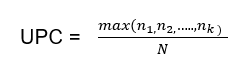
Where max (n1, n2,…nk) is the number of visits to the GP with whom the patient had the greatest number of visits, and N is the total number of visits by the patient to all providers during the same period. The UPC index reflects relational continuity with the same GP but does not capture continuity within a practice, which may also benefit patient care.
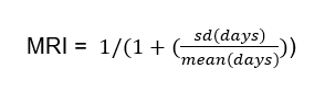
Regularity of GP care was measured using the Modified Regularity Index (MRI), which assesses the distribution of GP visits over time, based on the variation in the number of days between GP visits, with more even dispersion indicating better regularity (or planned, proactive care (Welsh et al 2023). MRI was calculated using the formula:
Both UPC and MRI were calculated for self-harm and comparison cohorts with at least three GP visits in the 12 months before the index date, ensuring sufficient data to accurately access continuity and regularity of care (Dreiher et al 2012). Both UPC and MRI result in scores ranging from 0 to 1. The UPC index was categorised into five groups: low (index range 0–0.49), moderate (0.5–0.74), high (0.75–0.99) and perfect (1) continuity and those without a UPC index categorised separately. For analysis, the UPC categories were then dichotomised into poor continuity (low and moderate) and high continuity (high and perfect). The MRI was categorised into quintiles (least to most regular), with an additional category for those without an MRI score. For analysis, the MRI quintiles were then dichotomised into poor regularity (quintiles 1-3) and high regularity (quintiles 4 and 5).
Statistical analysis
For the next stage of the analysis, differences in health service use over time between the self-harm and comparison cohort were examined using generalised estimating equations (GEE) (Kotz et al 2014; Liang and Zeger 1986).
Generalised estimating equations models were used to assess changes in health service use between the two cohorts over time. GEE models were selected as they are well suited for repeated measures and longitudinal data, accounting for within-person correlation across time points. Each individual contributed two time points: the 12 months before and the 12 months after the index date. GEE provides robust population-averaged estimates, even when data are correlated or not normally distributed, making it ideal for evaluating changes in health service use over time in a matched cohort study.
For binary outcomes (whether a health service was used or not), GEE models with logit link, binomial family, and exchangeable correlation structure was used to estimate odds ratios (ORs).
For count outcomes (number of health services used), GEE models with a log link, Poisson distribution and exchangeable correlation structure was used to estimate rate ratios (RRs). Models for count outcomes included the log of person-years at risk as an offset term to account for differing follow-up time.
From these models, three key estimates were derived:
- A pre-index OR or RR comparing health service use between cohorts in the 12 months before the index date
- A post-index OR or RR comparing health service use between cohorts in the 12 months after the index date
- An interaction OR or RR, representing the differential change in service use from before to after in the self-harm cohort relative to the comparison cohort.
Both unadjusted and adjusted models were estimated. Unadjusted models included only the main effects for cohort, time and their interaction. Adjusted models included the matching variables (age, sex, Socio-Economic Indexes for Areas and remoteness for SA2) and comorbidities (measured using the Rx-Risk and MACSS indices) to account for differences and baseline health (Mitchell and Cameron 2018).
This report included both unadjusted and adjusted (for age, sex, socioeconomic status, remoteness and co-morbidities) estimates from each GEE model. The model results showed the difference in health service use between the self-harm and comparison cohorts in the year before and after the hospital admission and the difference in change between the periods over time between the two groups.
The next component of the report used a statistical approach referred to as latent class analysis (LCA) to identify subgroups based on health service use patterns over a person’s year before and year after index hospital admission.
LCA was selected over other clustering methods (such as k-means, hierarchical clustering) due to its statistical robustness and model-based approach to identify health service use patterns. LCA provides objective fit statistics, estimates membership probabilities for class selection rather than forced classification, and better handles mixed data types, resulting in more reliable pattern identification. Studies have shown that LCA produces lower misclassification rates compared to traditional clustering methods, making it particularly suitable for identifying complex health service use patterns (Naldi et al 2020).
LCA is a data-driven model-based approach that identifies underlying subgroups (called latent classes or groups) based on multiple observed variables (indicators). Individuals are probabilistically assigned to the groups based on two model parameters estimated on a maximum-likelihood basis:
- group membership probabilities; and
- the means and variances of the indicator variables, conditional on group membership.
Groups of individuals sharing similar patterns of the means and variances of each indicator variable are identified and grouped. This enables the distinctness of each identified groups to be assessed and qualitatively described.
The groups reflect the average service use patterns of ex-serving members based on model-estimated probabilities as opposed to being determined through upper and lower service use bounds. Therefore, an ex-serving member in the medium user group has, on average, medium health service use across all of the analysed health services. However, it is possible that a person in the medium user group has higher use of one health service and lower use of another health service, as long as their service use is, on average, at a medium level.
LCA was performed separately for each cohort in both the year before and year after hospital admission to identify distinct service use profiles.
The best-fitting model with the optimal number of classes was selected using several criteria:
- relative fit statistics (Akaike Information Criterion and Bayesian Information Criterion)
- classification diagnostics (entropy values close to 1, average posterior probability of group membership > 0.7 for each group, odds of correct classification based on posterior probabilities > 5 for each group and close correspondence between each latent group’s estimated probability of group membership and the proportion of cohort classified to that group according to posterior probability of group membership)
- smallest group size greater than 5% of the sample
- substantive model interpretability and parsimony.
Models with 2-5 groups were tested, with the three-group solution selected as optimal based on clear distinction between groups, average posterior probabilities (APP) for each group greater than 0.8, high odds of correct classification for each group >5. The three groups identified were characterised according to volume of health service use: low, medium and high.
Group labels (low, medium and high users) were assigned post hoc based on the relative volume and pattern of service use across the six analysed health services (GP, specialist, allied health, ED, hospital and PBS services). These labels were not based on pre-specified cut-offs but were instead informed by the model-estimated posterior probabilities and mean counts of health services use within each latent group, based on the data-driven grouping of individuals with similar patterns and intensity of service use.
The final analytical process that was used in this research was to examine the transition patterns by comparing health service use patterns for the year before and year after index hospital admission. This focussed on simplifying the nine possible transitions by categorising them into four patterns (stable low, stable medium/high, increasing and decreasing). Multinomial logistic regression was then used to identify factors associated with these transition patterns of service use changes among the self-harm cohort using the stable low or stable medium/high classes as reference.