Australian Burden of Disease Study: Methods and supplementary material 2018

Estimating attribution to risk factors

The estimated contribution of a risk factor to disease burden is calculated by comparing the observed risk factor distribution with an alternative and hypothetical distribution (the counterfactual scenario).This could be an increase or decrease in levels of exposure, or changes in behaviour compared with what is currently observed in the population.

Theoretical minimum risk exposure distribution

In the ABDS 2018, as in previous burden of disease studies, a theoretical minimum risk exposure distribution (TMRED) scenario was adopted. This involved determining the hypothetical exposure distribution that would lead to the lowest conceivable disease burden.

For some risk factors, the choice of TMRED is obvious, as it involves no exposure to risk – for example, all people are lifelong non-smokers, or all people are highly active. However, for many risk factors, no exposure is not appropriate, either because it is physiologically impossible (for example, blood pressure, or body mass index or BMI), or because there are lower limits beyond which exposure cannot feasibly be reduced (for example, air pollution). In these cases, epidemiological evidence is used to determine the optimal level of exposure, which reflects either the lowest level at which a dose–response relationship can be observed within a meta-analysis of cohort studies, or the lowest risk factor exposure distribution observed globally (GBD 2019 Risk Factors Collaborators 2020). The counterfactual then becomes a narrow distribution around the optimal level. For example, based on a meta‑analysis of global studies, the counterfactual distribution for high body mass index is based on a population mean of a body mass index of
20–25 kg/m² with a standard deviation of 1.

In the ABDS 2018, the TMRED for physical activity was reduced to 4,200 METs (Metabolic Equivalent of Tasks) from 8,000. The TMRED for many of the dietary risks and air pollution also changed to be a single value instead of a range of values due to different methods for GBD 2019 (see Risk factor specific methods for TMREDs).

Where the TMRED is a range, exposure to risk is not dichotomous (that is, at risk or not at risk). In this situation, the measure of attributable burden cannot be estimated by simply comparing each level of exposure in the population with the endpoints. Instead, to determine how much burden each exposure level contributes compared with TMRED, the relative position in the range of the level of exposure is compared with its relative position in the range of the TMRED. The appropriate TMRED value for each category of exposure depends on the placement of their category within the risk factor exposure distribution of the population, starting at the lowest TMRED possible.

For example, if a persons’ BMI is in the range 26.0–27.9 kg/m² (category A) and the TMRED for that person is in the range 20–25 kg/m² then a TMRED value is estimated by comparing the median from category A with the proportion of the population with a BMI less than that median value. That is, the median within category A is a BMI of 27.0 kg/m² and this BMI is greater than 60% of the population’s BMI, the TMRED value for category A is equal to 60% of the possible TMRED values from within this range (20 kg/m² up to 25 kg/m²⁾. Assuming the TMRED distribution is uniform then the TMRED for category A is a BMI of 23.

This model assumes that a healthy BMI (the BMI levels not associated with disease outcomes) is a range, as opposed to a single value for the entire population. The level of risk of disease outcomes for each person in the population is then calculated, based on the level of actual BMI compared with the TMRED value from within the range.

Figure 3.2: Example of estimating the TMRED for a category of overweight and obesity

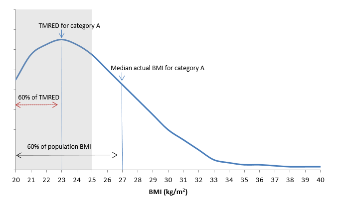
Note: The shaded range in the figure refers to the TMRED, which is between 20 kg/m² and 25 kg/m². Category A is the BMI of 26.0 to 27.9 and the median of this category is 27.0.

Population distribution of exposure

A clear and consistent definition of risk factor exposure is key to estimating the proportion of the population ‘at risk’. For the ABDS 2018, the definitions of risk factor exposures have been adopted where possible from the GBD 2019 (GBD 2019 Risk Factors Collaborators 2020) and the AIHW review of the literature (AIHW 2017a, 2017b, 2018).

All potential data sources to estimate exposure (whether published or unpublished) were assessed for comparability, relevance and representativeness, currency, accuracy, validation, credibility and accessibility/timeliness (see the data selection criteria and the scoring matrix). Only data sources that met these criteria were included in the study.

Estimates of Australian and Indigenous population distributions of risk factor exposure by age and sex have been based on a variety of data sources:

• ABS apparent consumption of alcohol data (national estimates only)
• ABS Labour force survey
• Australian Health Survey (AHS) 2011–12 (national estimates only)
• Australian Aboriginal and Torres Strait Islander Health Survey (AATSIHS) 2012–13 and National Aboriginal and Torres Strait Islander Health Survey (NATSIHS) 2018–19 (Indigenous estimates only)
• Census of population and housing
• National Drug Strategy Household Survey (NDSHS) 2019 (national estimates only)
• National Health Survey (NHS) 2017–18 (national estimates only)
• National HIV Register
• National Homicide Monitoring Program
• National Hospital Morbidity Database (NHMD)
• National Mortality Database (NMD)
• National Perinatal Data Collection (NPDC)
• National Perinatal Mortality Data Collection (NPMDC)
• Personal Safety Survey (PSS) 2016 (national estimates only)
• Safe Work Australia
• satellite modelled data calibrated to ground-based air monitoring stations
• The Kirby Institute annual surveillance reports
• epidemiological studies.

Some risk factors (such as illicit drug use) had several different measures or definitions of exposure. For illicit drug use, these included opioid use, amphetamine use, cannabis use, cocaine use, other illicit drug use as well as unsafe injecting practices. These different measures of exposure are mutually exclusive for illicit drug use and can be summed.

The risk factor exposure for comparative risk assessment is measured as either a categorical variable (with a set number of mutually exclusive categories) or a continuous variable.

Some categorical risk factors are measured through relatively straightforward dichotomous descriptions (for example, the proportion of people exposed to second-hand smoke versus the proportion who were not). For other risk factors, broad categories are used, such as the proportion of the population (by age and sex) falling into standardised categories of physical activity.

However, the majority of risk factors are measured as continuous variables, and the PAF calculations require the population prevalence per unit of exposure (for example, the observed population distribution of systolic blood pressure per millimetre of mercury), by age and sex.

Some previous burden of disease studies used a modelled risk exposure distribution rather than the empirical data themselves. They have, for example, taken the observed mean and standard deviation of exposure to a risk factor in the population, then modelled the exposure distribution using a normal or a lognormal function with that mean and standard deviation. This approach was used for the risk factors alcohol use and low bone mineral density.

For the ABDS 2018 study, empirical survey data were used where possible to determine the distribution of exposure to risk factors. The data were derived from the sources described in the risk factor specific methods. The proportion of the population exposed to each risk factor level was estimated in accordance with the finest exposure increments supported by the data source. Where there were no relevant updates to the data (such as data sourced from the AHS 2011–12) the survey data was modelled where possible to reflect the change over time to estimate exposure in 2018 as described for each risk factor.

Where data were extracted directly from a survey (for example, the National Health Survey 2017–18), sex, age and exposure categories were extracted at the finest possible level of granularity within an exposure distribution. Where necessary, categories were aggregated into larger cells to conform with requirements for the clearance of minimum cell sizes.

Estimates of effect size (relative risks)

Burden of disease studies use relative risks to measure the strength of causal association between risk factors and the linked disease outcomes. The ABDS 2018 adopted relative risks estimated by the GBD 2019 or the AIHW review of the literature (AIHW 2017a, 2017b, 2018; GBD 2019 Risk Factors Collaborators 2020). The GBD relative risks used were judged appropriate to be used globally, in different countries and for different ethnicities.

The relative risks from the GBD 2019 for infectious diseases such as hepatitis C, hepatitis B, HIV/AIDS and tuberculosis were not considered appropriate for Australia because control mechanisms exist in Australia for these conditions. They were estimated with direct evidence data as described for each risk factor in Risk factor specific methods.

Effect sizes used were adjusted for confounders (‘parallel’ risk factors), but not for factors that occur successively along the causal pathway. For example, relative risk of coronary heart disease due to physical inactivity was not adjusted for high blood plasma glucose, as these risk factors occur along the same causal pathway. This means the estimates of their effects cannot be added together.

For some continuous risk factors, the distribution of relative risks across the required levels of exposure were determined by applying a linear relationship to the available units of measure for each risk factor and the published relative risks by age and sex. However, exceptions were made for overweight (including obesity), which were determined by the literature (AIHW 2017b).

Where categories of relative risk did not correspond to an equivalent exposure category, the relevant relative risk to apply to each exposure category was determined as the relative risk for the median survey response of that category. For example, for the proportion of the population who had a blood pressure between 115–120 mmHg, the relative risk for the median, which is 117 g in this example, was applied. When the exposure category included an open-ended range, the median in this range was also used.

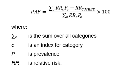
Calculation of population attributable fractions

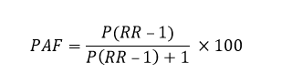
PAFs determine the proportion of a particular disease that could have potentially been avoided if the population had never been exposed to a risk factor (or, rather, had been exposed to TMRED levels). PAFs were calculated for each linked disease by year, sex and age group.

For most risk factors the calculation of PAF remained the same as previous ABDS studies. The calculation of PAFs requires the input of the relative risk (RR) and prevalence of exposure in the population (P):

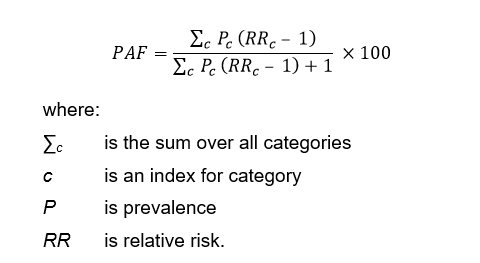
When the risk factor has multiple categories of relative risks and exposure levels, the following formula is used:

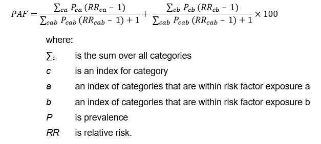
This formula is modified to produce separate estimates for risk factor exposures which are part of a continuous distribution, such as overweight, which is part of the risk factor overweight (including obesity). The PAF for overweight (including obesity) is the sum of the PAF for overweight (numerator includes the categories of exposure classified as overweight but not obese) and a PAF for obesity (numerator includes the categories of exposure classified as obese). The denominators for the PAFs includes categories for both overweight and obesity.

For selected risk factors, the PAF calculation formula was changed based on GBD 2019. This formula allows the relative risks to be protective and therefore less than 1. The risk factors using this formula are physical inactivity; diets low in vegetables, fruit, wholegrains, milk, nuts, and legumes; diets high in red meat, processed meat and polyunsaturated fats; and low birthweight & short gestation.

Direct population attributable fractions

For some risk–outcome pairs, direct evidence is used to calculate the PAF. This is used:

• for linked diseases where there is evidence from high-quality data sources to attribute a disease outcome to a risk factor in Australia. It is important that the estimate captures all cases of the disease outcome in Australia. An example is the HIV register, which collects data on the risk factor exposures that cause HIV (unsafe sex and/or drug use). The direct PAF is calculated as the proportion of the outcome caused by the risk factor.
• when the PAF is sourced from the GBD study where no relative risks are published because the GBD study has a cause which is the disease due to a risk factor, such as chronic liver disease due to alcohol use. The PAF is calculated using the burden for chronic liver disease due to alcohol use as a proportion of all burden due to chronic liver disease.
• when the PAF is sourced from ABDS disease burden estimates where sequela level burden is due to a risk factor, such as drug use disorders with components made up from individual drug dependence estimates. The PAF is calculated using the sequela burden from dependence for each drug (for example cannabis dependence) as a proportion of all burden due to drug use disorders.
• when exposure to the risk factor is necessary to have the outcome – for example, all of the disease outcome ‘alcohol use disorders’ is attributable to the risk factor ‘alcohol use’. In this case, the PAF is 1, where all of the disease outcome is attributed to the risk factor.

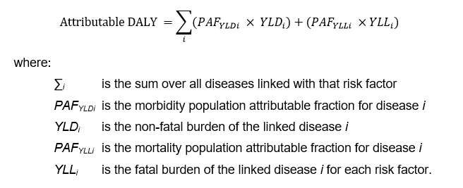
Calculating the attributable burden

Attributable DALY for each risk factor and linked disease is calculated at the disease level (for each age and sex), described mathematically as:

Applying PAFs to the ABDS disease list

A small number of linked diseases and injuries sourced from the GBD 2019 did not align to the ABDS disease list. This was due to the GBD disaggregating causes to a further level – for example, stroke, which was estimated as a single disease in the ABDS 2018, had only relative risks from the GBD 2019 for 3 sub-types of stroke (ischaemic stroke, subarachnoid haemorrhage and intracerebral haemorrhage). These could not be applied directly to the single stroke burden.

To adjust for this, data were used from a range of sources to identify the proportion of the prevalence of the ABDS disease corresponding to the available relative risk. For example, Thrift et al. (2009) found ischaemic stroke to be 77.6% of strokes in Australia. Where such disaggregation was unavailable from published literature, the proportion of fatal/non-fatal burden for these diseases in Australia from the GBD 2019 was used. The table below describes the source of any such disaggregation and the proportion used.

Note: Percentages may not sum to 1 due to rounding.

A limitation of this approach is that the proportion of prevalence does not always equate to the proportion of the burden represented by the GBD cause, and this might vary by fatal and non-fatal burden.

The PAFs for each risk factor were calculated at the GBD cause level (disaggregated level). The PAFs were multiplied by the proportion of the ABDS disease it represented and applied at the ABDS disease level to calculate the attributable YLD, YLL and DALY. For example, the PAFs for ischaemic stroke were multiplied by 0.776 before being used to calculate the attributable DALY.

Combined risk factor analysis

The burden from different risk factors for a particular disease cannot simply be added together, because:

• some risk factors are on the same causal pathway – for example, a diet high in sodium increases the likelihood of high blood pressure
• the PAFs are estimated independently – similar to issues with comorbidity, the burden due to each risk factor for a given disease might exceed the total burden of that disease.

The combined effect of multiple risk factors must account for the bias introduced by the complex pathways and interactions between many risk factors.

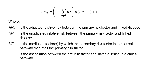
Firstly, to account for risk factors on the same causal pathway, mediation factors were used to attenuate the relative risk for the risk factor first in the pathway which mediate through the second risk factor in the same causal pathway for the linked disease. The relative risks for the first risk factor and the linked disease are reduced as the burden is already attributed to the risk factor/s secondary in the causal pathway. When multiple risk factors are possible secondary causal pathways for the linked disease, the attenuation factors were summed (see figure below). The attenuation factors were sourced from the GBD 2019 (GBD 2019 Risk Factors Collaborators 2020).

For example, to reflect the causal pathway of a diet low in fruit increasing the risk of stroke, mediation accounted for the diet’s causal pathway towards increasing the risk of three other risk factors, which each, in turn, increase the risk of stroke.

Figure 3.3: Example of associations between a primary risk factor and linked diseases mediated by secondary risk factors in a causal pathway

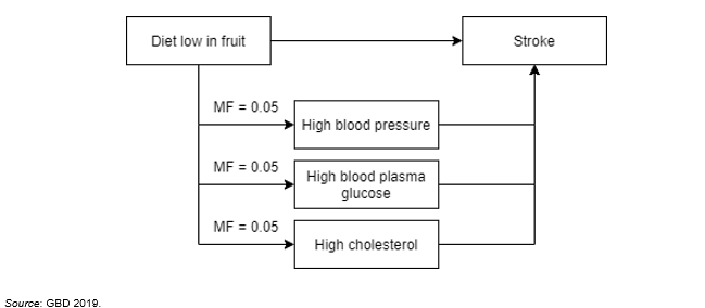
The amount of mediation of a diet low in fruit causing high blood pressure and then stroke was estimated to be 5% by the GBD 2019. This was summed with the mediation factors for high blood plasma glucose and high cholesterol. The relative risk for a diet low in fruit causing stroke was therefore mediated by 15%. These were then used to calculate adjusted PAFs to provide the necessary independence assumption required for the next step.

Following mediation, to prevent the combined disease burden’s exceeding the total burden for a given disease, the combined burden of more than 1 risk factor was estimated using the following joint effect formula:

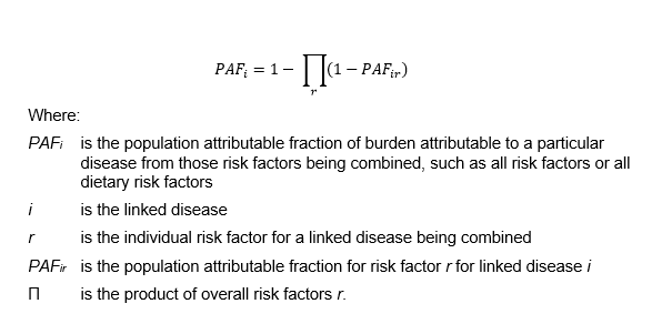
This formula, which has been used in several other studies, has the desirable property of placing a cap on the estimated combined attributable burden, and thus avoids the possibility of exceeding 100% of the total burden of disease. However, it assumes that risk factors are independent – that is, it does not take into account risk factors that are in the same causal pathway.

The use of both the joint effect and mediation formulae therefore adjusts for the interrelatedness between risk factors in the same causal pathway as well as the combined impact of all risk factors and dietary risk factors included in the study.

Attributable burden estimates by socioeconomic group

The burden attributable to risk factors was estimated by socioeconomic group in 2015 and 2018. The risk factors were not estimated by state or remoteness as this was not in scope for this project. It was not possible to estimate exposure to the risk factors bullying victimisation, child abuse & neglect, low birth weight & short gestation, low bone mineral density, iron deficiency, sun exposure and unsafe sex by socioeconomic group.

For some risk factors, modelling was used to estimate exposure by socioeconomic group from the relevant survey. This is due to high RSEs when trying to estimate directly from the relevant survey. For these risk factors, exposure by socioeconomic group was estimated by comparing the mean estimate of exposure in each quintile and the mean national exposure from the survey by age and sex. The absolute change between these estimates was then used to adjust unit record data to reflect exposure to the risk factor in each socioeconomic group.

The methods for each risk factor are described in Risk factor specific methods.

2015, 2011 and 2003 estimates

Where possible the burden attributable to risk factors was calculated for 2015, 2011 and 2003. Exposure distributions for air pollution was estimated only for 2018 and 2015 as PM2.5 (particulate matter 2.5) estimates from satellite data was not available for the other years. Exposure to high plasma glucose could not be estimated in 2003. Bullying victimisation, child abuse & neglect, low bone mineral density, iron deficiency and sun exposure PAFs were based on data relevant to the whole period of the study and were considered appropriate for 2003, 2011 and 2015. The new risk factor low birth weight & short gestation was only estimated in 2018.

The way exposure was estimated for risk factors in 2015, 2011 and 2003 is described in the individual risk factor section in Risk factor specific methods.

Changes in risk factor exposure over time

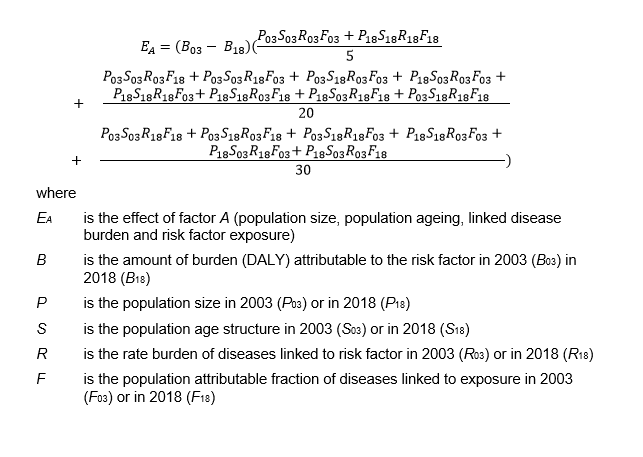
The Das Gupta method was used to decompose the changes in burden attributable to each risk factor into 4 additive components (Das Gupta 1993). Using a series of scenarios, this method calculates the effect of each factor on the changes over time by assuming that all other factors, except the factor under consideration, remain the same at both time points.

The change in overall attributable burden is decomposed into changes due to:

• population growth – in Australia population size is increasing over time
• population ageing – in Australia the proportion of older people is increasing over time
• risk factor exposure – changes in the prevalence of exposure to the risk factor in Australia.
• Changes in linked disease burden – changes in the overall burden for those diseases or injuries that are linked to the selected risk factor. This may be influenced by changes in diagnosis, treatment or health intervention (resulting in changes in disease prevalence or severity), as well as changes in other risk factors. For example, increases in overweight (including obesity) may have some impact on coronary heart disease burden which is also linked to tobacco use.

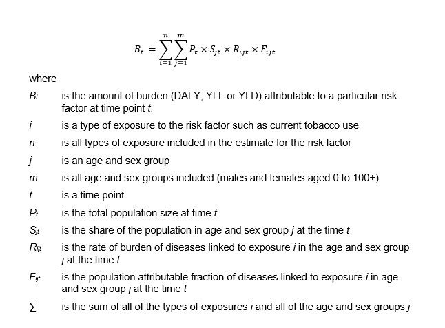
Attributable burden is estimated as the product of these 4 factors using the formula when examining burden by type of exposure to the risk factor:

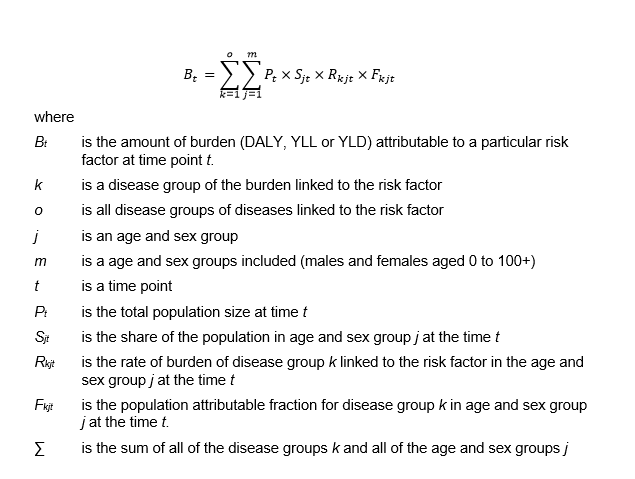
Attributable burden is estimated as the product of these 4 factors using the formula when examining burden by linked disease group:

The effect of each of the 4 factors – population size, population ageing, linked disease burden and risk factor exposure – using this method on the change in attributable burden between 2003 and 2018 is calculated as:

Indigenous estimates

For the Indigenous population, the same risk factor list was used as for the total Australian population, with 3 exceptions: unimproved sanitation, which was included for Indigenous estimates only; and high sun exposure and bullying victimisation, which were included for national estimates only. The burden from unimproved sanitation was not estimated for the non-Indigenous population due to lack of available exposure data, and was assumed to be close to 0. The burden from sun exposure was not estimated for the Indigenous population as it was not possible to account for the impact of differences in skin melanin levels. The burden from bullying victimisation was not estimated for the Indigenous population as data were not available to estimate exposure in a comparable way. The additional impacts of racism for Aboriginal and Torres Strait Islander people would also need to be taken into account. The AIHW is exploring this issue further with the view to incorporating a measure of bullying and/or racism in future Indigneous burden of disease studies.

The same risk–outcome pairs, relative risks and TMREDs as used for national estimates were used for Indigenous risk factor estimates. Relative risks specific to the Indigenous population were not available.

Exposure distributions for some risk factors could not be measured for the 2003 Indigenous estimates due to lack of available input data comparable with the methods used for the 2011 and 2018 estimates. These were air pollution, high blood plasma glucose, unimproved sanitation, and low birthweight & short gestation. As a result, these risk factors were not included in the 2003 Indigenous estimates.